Note
Go to the end to download the full example code.
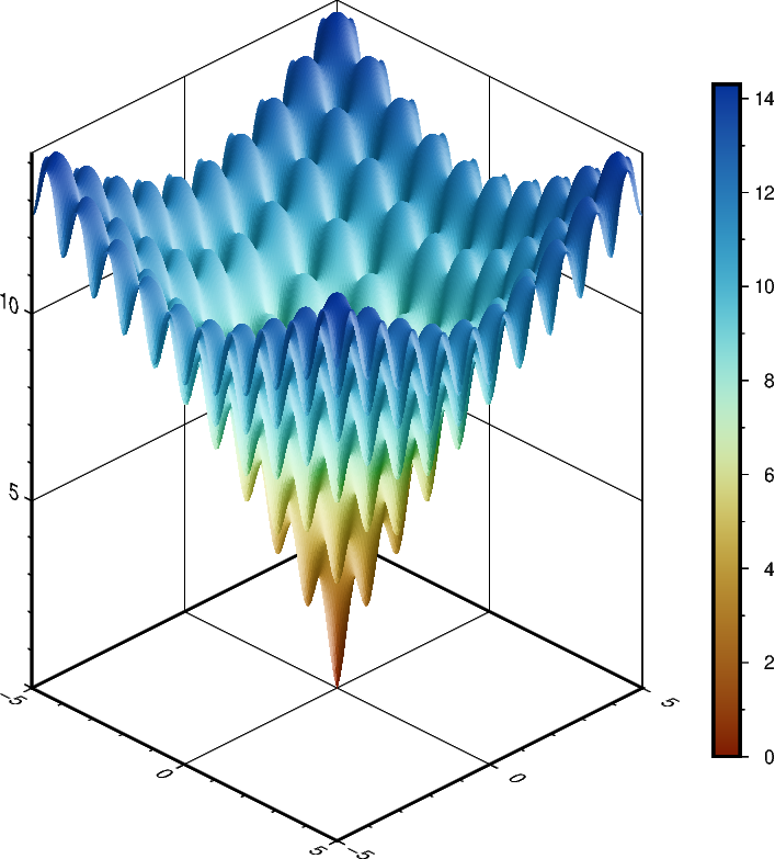
Plotting a surface
The pygmt.Figure.grdview method can plot 3-D surfaces with
surftype="surface". Here, we supply the data as an xarray.DataArray with
the coordinate vectors x and y defined. Note that the perspective parameter
here controls the azimuth and elevation angle of the view. Specifying the same scale
for the projection and zscale parameters ensures equal axis scaling. The
shading parameter specifies illumination; here we choose an azimuth of 45° with
shading="+a45".
import numpy as np
import pygmt
import xarray as xr
from pygmt.params import Axis, Frame, Position


# Define an interesting function of two variables, see:
# https://en.wikipedia.org/wiki/Ackley_function
def ackley(x, y):
    """
    Ackley function.
    """
    return (
        -20 * np.exp(-0.2 * np.sqrt(0.5 * (x**2 + y**2)))
        - np.exp(0.5 * (np.cos(2 * np.pi * x) + np.cos(2 * np.pi * y)))
        + np.exp(1)
        + 20
    )


# Create gridded data
INC = 0.05
x = np.arange(-5, 5 + INC, INC)
y = np.arange(-5, 5 + INC, INC)
data = xr.DataArray(ackley(*np.meshgrid(x, y)), coords=(x, y))

fig = pygmt.Figure()

# Plot grid as a 3-D surface
SCALE = 0.5  # in centimeters
fig.grdview(
    data,
    # Set annotations and gridlines in steps of five, and tick marks in steps of one
    frame=Frame(
        axis=Axis(annot=5, tick=1, grid=5),  # x and y axes
        zaxis=Axis(annot=5, tick=1, grid=5),
    ),
    projection=f"x{SCALE}c",
    zscale=f"{SCALE}c",
    surftype="surface",
    cmap="SCM/roma",
    perspective=[135, 30],  # Azimuth southeast (135°), at elevation 30°
    shading="+a45",
)

# Add colorbar for gridded data in the Middle Right corner.
fig.colorbar(annot=2, tick=1, position=Position("MR", cstype="outside"))

fig.show()
Total running time of the script: (0 minutes 2.717 seconds)